Vertex Cover

Definition

We are given an undirected graph with vertex set $V$ and edge set $E$.

Our aim is to find the smallest number of nodes to be coloured, such that every edge has a coloured vertex. Also, which vertices would these be?

Applications

The Vertex Cover has applications in matching problems and optimization problems in fields like Biochemistry, Computational Biology, Monitoring and Computer Network Security.

Path to solving the problem

Vertex Cover is a minimization problem and its cost function can be cast to a QUBO problem through its respective Hamiltonian (see the Introduction and a reference),

$$ \displaystyle \large H = A \textstyle\sum\limits_{uv \in E} (1 - x_u) (1 - x_v) + B \textstyle\sum\limits_{v} x_v $$

where $A$ and $B$ are positive constants, $u, v \in V$ and $x_u$ is a binary variable, which is $1$ if vertex $u$ is part of the Vertex Cover and $0$ if it is not. For a valid encoding, the $A$ and $B$ constants need to obey the relation $A > B$. Otherwise, if this rule is not followed, the spin configuration for the lowest energy $H$ may not correspond to the best solution of our Vertex Cover problem or even to a valid one. At the same time $A \gg B$ would not be desired, as it would cause a large energy separation in $H$, impeding our solution approach.

Qaptiva HPC allows us to encode a problem in this Hamiltonian form by using the VertexCover class for a given graph and constants $A$ and $B$. We can then create a job from the problem and send it to a Simulated Annealer (SA) wrapped with a Quantum Processing Unit (QPU) interface. The SA will minimize the Hamiltonian, hence we find the solution to our problem.

In fact, the QLM contains an even more powerful solver $-$ Simulated Quantum Annealing (SQA). This quantum annealer has been tested on numerous benchmarks for the NP problems supported and produces results with a quality usually exceeding $98\%$. More details can be found in the documentation.

Quantum complexity

To represent the problem as QUBO, myQLM would need $N$ spins $-$ to encode each of the $N$ vertices.

Example problem

Imagine we are given a graph with $6$ vertices and $6$ edges, as shown below (left). The solution of this problem is quite easy to guess $-$ we can simply colour node $0$ and either node $1$ or node $5$ (right).

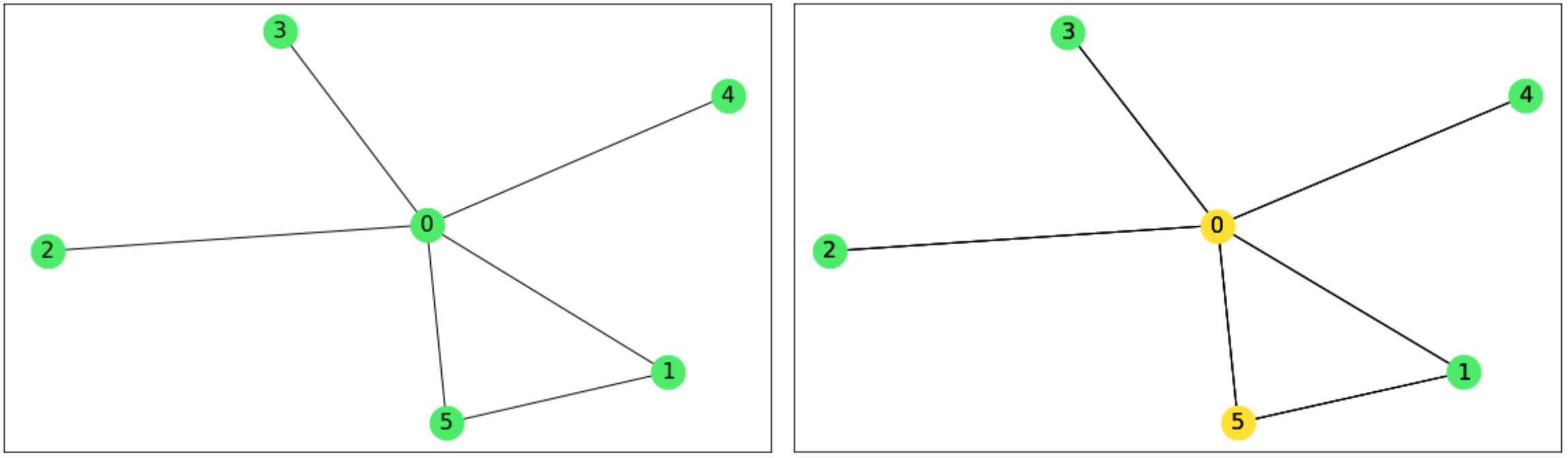
However, let's describe a method, which will enable us to find the Vertex Cover of any graph!

We shall start by specifying a graph with the networkx library along with the constants $A$ and $B$.

import networkx as nx
import numpy as np
import matplotlib.pyplot as plt

# Specify the graph 
# First example
graph = nx.Graph()
graph.add_nodes_from(np.arange(6))
graph.add_edges_from([(0, 1), (0, 2), (0, 3), (0, 4), (0, 5), (1, 5)])

# # Second example
# graph = nx.gnm_random_graph(15, 20)

# Impose constraints for the right encoding
B = 1
A = B + 0.01

# Draw the graph
nodes_positions = nx.spring_layout(graph, iterations=len(graph.nodes())*60)
plt.figure(figsize=(10, 6))
nx.draw_networkx(graph, 
                 pos=nodes_positions, 
                 node_color='#4EEA6A', 
                 node_size=440, 
                 font_size=14)
plt.show()

Once the graph is specified and the constants $A$ and $B$ correctly chosen, we can encode the problem via our VertexCover class:

from qat.opt import VertexCover

vertex_cover_problem = VertexCover(graph, A=A, B=B)

Solution

Resolution of the problem using a BatchGenerator

A high level solver of the VertexCover problem is available in the QLM under the form of a BatchGenerator called VertexCover. It is designed as simple interface to solve the problem on an input graph, while hiding the complexities of the underlying algorithms.

The different resolution methods that can be selected are "qaoa" (for QAOA Circuit Generation), "annealing" (for Simulated Quantum Annealing), and "schedule" (for Analog Quantum Scheduler Generation). A user-interpretable result is returned from the job execution, where the two resulting partitions of the nodes and the number of edges cut can be retrieved from the subsets and cost attribute respectively. A display method is also provided by the result object to visualize the partitioning of the graph.

An example of using the batch generator to generate a quantum annealing job and executing it with SimulatedAnnealing is provided below.

from qat.generators import VertexCoverGenerator
from qat.qpus import SimulatedAnnealing
from qat.core import Variable

# 1. Extract parameters for SA
problem_parameters_dict = vertex_cover_problem.get_best_parameters()
n_steps = problem_parameters_dict["n_steps"]
temp_max = problem_parameters_dict["temp_max"]
temp_min = problem_parameters_dict["temp_min"]

# 2. Create a temperature schedule and a QPU
tmax = 1.0
t = Variable("t", float)
temp_t = temp_min * (t / tmax) + temp_max * (1 - t / tmax)

vertex_cover_application = VertexCoverGenerator(job_type="sqa") | SimulatedAnnealing(temp_t=temp_t, n_steps=n_steps)
combinatorial_result = vertex_cover_application.execute(graph, A, B)

print("The nodes in the subgraph that forms a cover are", combinatorial_result.cover)
print("The number of nodes in the cover is", len(combinatorial_result.cover))

combinatorial_result.display(with_figure=True, figsize=(10, 6), node_size=440, font_size=14, pos=nodes_positions)

The nodes in the subgraph that forms a cover are [0, 1]
The number of nodes in the cover is 2

Simulated Annealing

If we want to solve the problem with SA straight, we can still do so via the following steps:

1. Extract some fine-tuned parameters for VertexCover (found for SQA) which are needed for the temperature schedule.

2. Create the temperature schedule using the t time variable (instance of the class Variable) and thus the SimulatedAnnealing QPU.

3. Create a job from the problem by calling the to_job() method and send it to the QPU.

4. Extract the Result and present the solution spin configuration.

5. Show the graph with the coloured nodes.

Each spin from the solution configuration corresponds to a node from the graph at the same position. Note that if the numbering of the input nodes starts from $1$ and not from $0$, one still needs to look at the $0$th spin to extract information for this first node, numbered as $1$.

When a spin has the value of $1$, this means that the respective node should be coloured and is part of the Vertex Cover.

from qat.qpus import SimulatedAnnealing
from qat.simulated_annealing import integer_to_spins
from qat.core import Variable

# 1. Extract parameters for SA
problem_parameters_dict = vertex_cover_problem.get_best_parameters()
n_steps = problem_parameters_dict["n_steps"]
temp_max = problem_parameters_dict["temp_max"]
temp_min = problem_parameters_dict["temp_min"]

# 2. Create a temperature schedule and a QPU
tmax = 1.0
t = Variable("t", float)
temp_t = temp_min * (t / tmax) + temp_max * (1 - t / tmax)
sa_qpu = SimulatedAnnealing(temp_t=temp_t, n_steps=n_steps)

# 3. Create a job and send it to the QPU
problem_job = vertex_cover_problem.to_job('sqa', tmax=tmax)
problem_result = sa_qpu.submit(problem_job)

# 4. Extract and print the solution configuration
state = problem_result.raw_data[0].state.int  # raw_data is a list of Samples - one per computation
solution_configuration = integer_to_spins(state, len(graph.nodes()))
print("Solution configuration: \n" + str(solution_configuration) + "\n")
indices_spin_1 = np.where(solution_configuration == 1)[0]
number_of_colours = len(indices_spin_1)
print("One would need to colour " + "\033[1m" + str(number_of_colours) + 
      "\033[0;0m" + " vertices, which are:\n" + str(indices_spin_1) + "\n")

# 5. Show the coloured graph
plt.figure(figsize=(10, 6))
node_size = 440
font_size = 14
nx.draw_networkx(graph, 
                 pos=nodes_positions, 
                 nodelist=indices_spin_1.tolist(), 
                 node_color='#FFE033', 
                 node_size=node_size, 
                 font_size=font_size)

indices_spin_minus_1 = np.where(solution_configuration == -1)[0]
nx.draw_networkx(graph, 
                 pos=nodes_positions, 
                 nodelist=indices_spin_minus_1.tolist(), 
                 node_color='#4EEA6A', 
                 node_size=node_size, 
                 font_size=font_size)
nx.draw_networkx_edges(graph, pos=nodes_positions)
plt.show()

/tmp/ipykernel_3933/2191584382.py:18: UserWarning: If SQAQPU is used, gamma_t will be needed.
  problem_job = vertex_cover_problem.to_job('sqa', tmax=tmax)

Solution configuration: 
[ 1. -1. -1. -1. -1.  1.]

One would need to colour 2 vertices, which are:
[0 5]

Solution analysis

For graphs which are quite big, one may find it hard to examine visually the solution. Therefore, here is a simple check for this purpose $-$ whether each edge has a coloured vertex and if not $-$ a list of colourless edges.

colourless_edges_list = []
for (node_i, node_j) in graph.edges():
    if node_i not in indices_spin_1 and node_j not in indices_spin_1:
        colourless_edges_list.append((node_i, node_j))
if len(colourless_edges_list) == 0:
    print ("The graph is covered well !")
else:
    print("The " + "\033[1m" + str(len(colourless_edges_list)) + 
          "\033[0;0m" + " edges without coloured nodes are:")
    print("(node, node)")
    for edge in colourless_edges_list: print(edge)

The graph is covered well !