qat.qpus.MPSTraj

class qat.qpus.MPSTraj(hardware_model: HardwareModel | None = None, bond_dimension: int | None = None, n_steps: int = 100, n_samples: int | None = None, n_procs: int = 1, sim_method: str = 'number_discrete', initial_state: MPS | None = None, monitor_times: List[float] | None = None, monitor_function: Callable[[MPS], Dict[str, Any]] | None = None, shift_jump_ops: float | List[float] = 0.0, homodyne_phase: float | None = None, jump_rtol: float = 0.001, intrastep_bond_dim: int = 2, disable_resource_management: bool = False, seed: int | None = None)

QPU for emulation of noisy analog quantum computing based on the quantum trajectory algorithm and MPS representation of statevectors.

This solves the following Lindblad equation:

\[\frac{d\rho}{dt} = -i[H, \rho] - \sum_k \left(\frac{1}{2} \{L_k^\dagger L_k, \rho\} - L_k \rho L_k^\dagger \right)\]

where \(H\) is the hamiltonian (given in the schedule), and the \(L_k\) are jump operators.

A Monte Carlo method known as the quantum trajectory method (see https://doi.org/10.1080/00018732.2014.933502 for a review) is used to solve it: a population of pure states, represented as MPS, is evolved under a random dynamics that reproduces the Lindblad equation above.

Several versions of the trajectory algorithm are implemented:

• Jump algorithm with discretized time (‘number_discrete’): a simple but biased method relying on time discretization.

• Jump algorithm with continuous time (‘number_continuous’): an unbiased version, with exact jump locations

• Homodyne algorithm (‘homodyne’): a quantum state diffusion method that avoids sharp jumps. It depends on a phase.

• Vovk-Pichler algorithm (‘vovk_pichler’): dynamically choose the homodyne or jump algorithm to minimize entanglement growth.

Parameters:

• hardware_model (HardwareModel) – A hardware model containing jump operators. Time-dependent jump operators and stochastic parameters are not supported yet. Defaults to None, i.e. noiseless dynamics.

• bond_dimension (int) – maximum bond dimension for MPS. At the end of each time step, the bond dimensions of the MPS are truncated to this value. Defaults to None, i.e. infinity.

• n_steps (int) – number of time steps. Defaults to 100.

• n_samples (int) – number of quantum trajectories. Defaults to 100. Ignored if the simulation is noiseless (single trajectory).

• n_procs (int) – max number of processes for multiprocessing. Default to 1, i.e. no multiprocessing.

• sim_method (string) – one of ‘number_discrete’ (default), ‘number_discrete_vp’, ‘number_continuous’, ‘homodyne’, ‘vovk_pichler’

• initial_state (StateMPS) – the initial state of the system given as a MPS. Overwrite the one given in the job.

• monitor_times (list<float>) – intermediate times at which to evaluate observables. The outcomes are returned as metadata.

• monitor_function (function of StateMPS returning dict<str, <scalar or array>>>) – Called along the simulation to produce output. Its only argument is the current state in MPS form. Must return a dictionary, each entry being a different quantity (scalar or numpy array). With Qaptiva access, it cannot depend on variables defined outside its scope.

• jump_rtol (float) – tolerance (relative to the time step) for finding jump location. For continuous algorithm only. Default is 1e-3.

• intrastep_bond_dim (int) – allows the bond dimension to increase beyond bond_dimension within a time step, by a factor intrastep_bond_dim. By default the bond dimension can grow 16-fold the base truncation value before truncation is performed to bring it back to the base value. This avoids overhead caused by performing SVDs at each operator application, in particular dor non-1D hamiltonians.

• shift_jump_ops (float or list<float>) – if set, this scalar value is removed from the jump operators, and the hamiltonian is compensated accordingly. This solves the same equation, but can dramatically change performances. If a list is given, this gives a different shift for each jump operator.

• homodyne_phase (float) – phase for the homodyne algorihtm. It also set the phase of any homodyne steps performed with the Vovk-Pichler method.

• disable_resource_management (bool) – default to False.

• seed (int) – set the seed of the random number generator. Only one trajectory is allowed in that case.

Notes

• all arguments are optional

• The schedule must represent a unitary evolution.

• In Sample mode, the number of trajectories is capped by the number of shots.

n_procs

Number of processes to run trajectories in parallel.

Type:

int

jump_ops

Jump operators, after appplying shift.

Type:

list of Observable

ham_shift

Extra contribution to hamiltonian due to jump operators shift.

Type:

Observable

Mathematical description

MPSTraj performs a trajectory algorithm to solve the following Lindblad equation:

\[ \begin{align}\begin{aligned}\frac{d\rho}{dt} &= \mathcal{L}[\rho]\\\mathcal{L}[\rho] &= -i[H, \rho] + \mathcal{D}[\rho]\\\mathcal{D}[\rho] &= - \sum_k \left(\frac{1}{2} \{L_k^\dagger L_k, \rho\} - L_k \rho L_k^\dagger \right)\end{aligned}\end{align} \]

where \(H\) is a potentially time-dependent hamiltonian and \(L_1, L_2, \ldots\) are arbitrary (static) jump operators. Note that MPSTraj also works without jump operators, in which case it computes the unitary dynamics given by \(H\), and is then an analog version of qat.qpus.MPS.

Trajectory algorithm

To emulate this dynamics, we use a stochastic method called the trajectory algorithm [Daley2014] [Plenio1998]. The lindbladian evolution is first trotterized into a succession of quantum channels. At each time step corresponds a channel, from which one Krauss operator is chosen at random and applied to the state. The number of time steps is given by the argument n_steps. A trajectory is thus a random choice of a succession of Krauss operators applied to the initial pure state. By folowing this method, we represent the (mixed) state of the quantum computer \(\rho\) as a distribution of pure states:

\[\rho = \sum_{\phi} p_{\phi} | \phi \rangle \langle \phi |\]

thus avoiding the memory-intensive storage of the density matrix. Averaging over trajetories allows to recover observables:

\[\langle O \rangle = \sum_{\phi} p_\phi \langle \phi | \hat O | \phi \rangle\]

In practice, we need to take a finite number \(N_t\) of such trajectories (given by n_samples), to approximate the density matrix. The error we make by doing so decreases as \(1 / \sqrt{N_t}\), as expected for a Monte-Carlo algorithm. One typically take \(N_t \sim 10^2\textrm{-}10^4\), but this will depend on the noise level, the simulation method and the exact dynamics simulated. Another advantage of the trajectory algorithm is that trajectories are independent from each other, and can thus be run in parallel in a straightforward manner. The number of parallel processes to use is imposed by the parameter n_procs.

Matrix Product States

To increase efficiency even more, the pure states are stored as Matrix Product States (MPS), which are particularly efficient at compressing lowly entangled states [Schollwock2011].

A MPS is a tensor network whose dimensions grow as trotter steps are applied to it. To keep memory and performance in check, it is regularly compressed. The compression level is given by a bond dimension \(\chi\) (through the argument bond_dimension). The higher \(\chi\) is, the more accurate the MPS representation of the state, at a cost of an increased memory footprint (scaling as \(\chi^2\)) and computation time (scaling as \(\chi^3\)). The compression brings in an approximation which is controlled by the amount of entanglement entropy \(S\) of the state. The approximation error is negligible when \(\chi \gg e^S\) at all time. The MPS is kept in a so-called canonical form, to ensure quick computation of norm and observables, as well as optimal compressions.

For better performances, wihtin a trotter step, the bond dimension is allowed to go beyong \(\chi\) by a multiplying factor given by intrastep_bond_dim, which is 2 by default. Adapting this parameter may bring performance gains for schedules with a 2D connectivity or more, due to the increased cost of the canonicalization procedure, which is necessary before compression.

See qat.qpus.MPS for more details on MPS, and [Bonnes2014] for details on using MPS in trajectory algorithms.

Choice of unraveling

We mentionned earlier that each trotter step is a quantum channel, which we write with Kraus operators. There is a freedom in expressing a quantum channel with Krauss operators, called an unraveling [Breuer2007], and MPSTraj allows several options through the parameters method_sim.

• The method number_discrete implements the standard jump algorithm, with discretized time steps. The dissipative part of the lindbladian is written with two Kraus operators:

  \[ \begin{align}\begin{aligned}\exp(dt \mathcal{D})[\rho] &= \sum_{i=0,1} K_i \rho K_i^\dagger + O(dt^2)\\K_0 &= \exp\left(- \frac{dt}{2} L^\dagger L\right)\\K_1 &= \sqrt{dt} L\end{aligned}\end{align} \]

• The method homodyne implements the homodyne method, also called quantum state diffusion [Percival1998]. The dissipative part of the lindbladian is represented as a continuum of Kraus operators:

  \[ \begin{align}\begin{aligned}\exp(dt \mathcal{D})[\rho] &= \int d\xi P_{\rm norm}(\xi) K(\xi) \rho K(\xi)^\dagger + O(dt^2)\\K(\xi) &= \exp\left(-\frac{dt}{2} L^\dagger L\right) + e^{i\phi} L \xi\end{aligned}\end{align} \]

  where \(P_{\rm norm}(\xi)\) is the random distribution of \(\xi\) and is gaussian, centered around \(\xi_0 = \langle e^{i\phi} L + e^{-i\phi} L^\dagger \rangle dt\), and of variance \(dt\). This representation is parameterized by a phase \(\phi\), specified in the parameter homodyne_phase.

• The method vovk_pichler is an adaptive method that automatically choose an unraveling that minimizes the growth of entanglement, at the cost of a small computation overhead (constant with number of qubits) at each time step. This implements the idea of Ref. [Vovk2022]. The optimal unraveling turns out to always be of the jump or homodyne type.

• The method number_continuous is a variant of number_discrete that pinpoints the precise (up to a tolerence given by jump_rtol) location of each jump on the time axis. This eliminates a bias \(O(dt)\) caused by the trotterization of the dissipative part of the Lindbladian. It is still subject to a trotter error coming from the unitary dynamics.

Finally, a last degree of freedom exists for the unraveling of the Lindblad equation. Jump operators can be shifted by a complex scalar \(\alpha\), leaving the Lindbladian invariant if the hamiltonian is adjusted accordingly:

\[ \begin{align}\begin{aligned}L_k &\rightarrow L_k - \alpha_k\\H &\rightarrow H + \frac{i}{2}\sum_k \left( \alpha_k L_k^\dagger - \alpha_k^* L_k \right)\end{aligned}\end{align} \]

This can be done through the parameter shift_jump_ops.

Performances

Thanks to its use of MPS, MPSTraj is able to reach much higher number of qubits than exact emulators such as qat.qpus.AnalogQPU. We show an example with up to 80 qubits.

To give an idea of performances, we simulate the quantum adiabatic preparation of the Maximum Independent Set (MIS) of a random graph with a Rydberg atom quantum computer. We assume a hamiltonian

\[H = -\delta(t) \sum_i n_i + \Omega(t) \sum_i X_i + U \sum_{\langle i, j \rangle} n_i n_j\]

with \(\delta(t)\) and \(\Omega(t)\) two controllable time-dependent parameters, \(U\) the strength of the Rydberg interaction. The interaction is assumed to be present only on pairs of nodes with an edge. The graph is a Unit-Disk (UD) connected random graph, similar to this one:

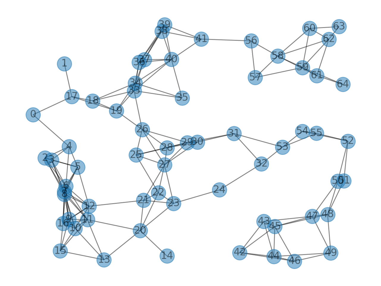
An example of random, connected, unit-disk graph used in this benchmark.

We look at the approximation ratio of the corresponding MIS problem obtained at the end of the adiabatic schedule with noiseless qubits, and under a dephasing noise of rate \(0.01 \Omega_\textrm{max}\). The result is shown in this figure:

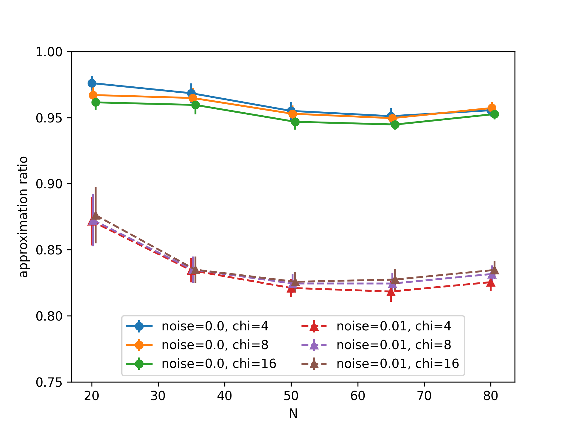
Simulation of solving MIS problems with an adiabatic evolution.

Error bars correspond to the cumulation of the trajectory sampling error (we took 100 trajectories) and the standard deviation over 10 random graphs. Increasing the bond dimension \(\chi\) does not change much the result, particularly in the noisy case, showing that entanglement is well captured by the MPS at these values of \(\chi\).

The runtime of these simulation is shown below.

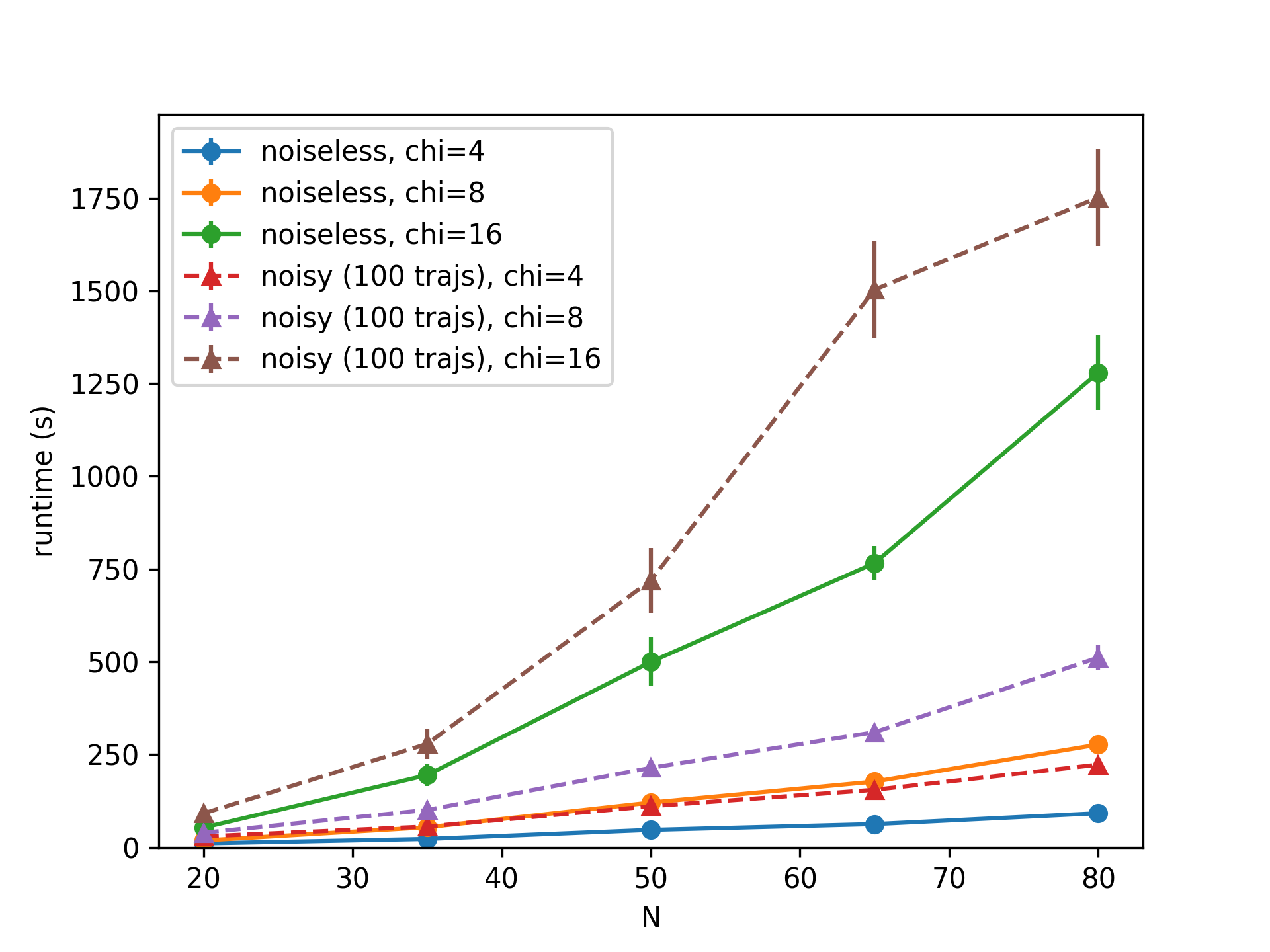
Simulation runtime for increasing number of qubits \(N\) and bond dimension \(\chi\). Noisy simulations are paralellized over 50 CPUs. Average over 10 graphs.

Computation time increases polynomialy with the number of qubits \(N\), but exponentially with the bond dimension \(\chi\). Noisy simulations are performed with 100 trajectories spread between 50 CPUs. The largest calculation took about 30 minutes.

Below we show the runtime of emulating a standard quantum annealing schedule for preparing antiferromagnetic states in Rydberg atom systems, in the absence of noise. For a 1D chain of \(N\) atoms, entanglement is very low (area law), so that a bond dimension as low as \(\chi=2\) is almost exact. In that case we see a wall time that grows linearly with \(N\), to be compared to an exponential for AnalogQPU.

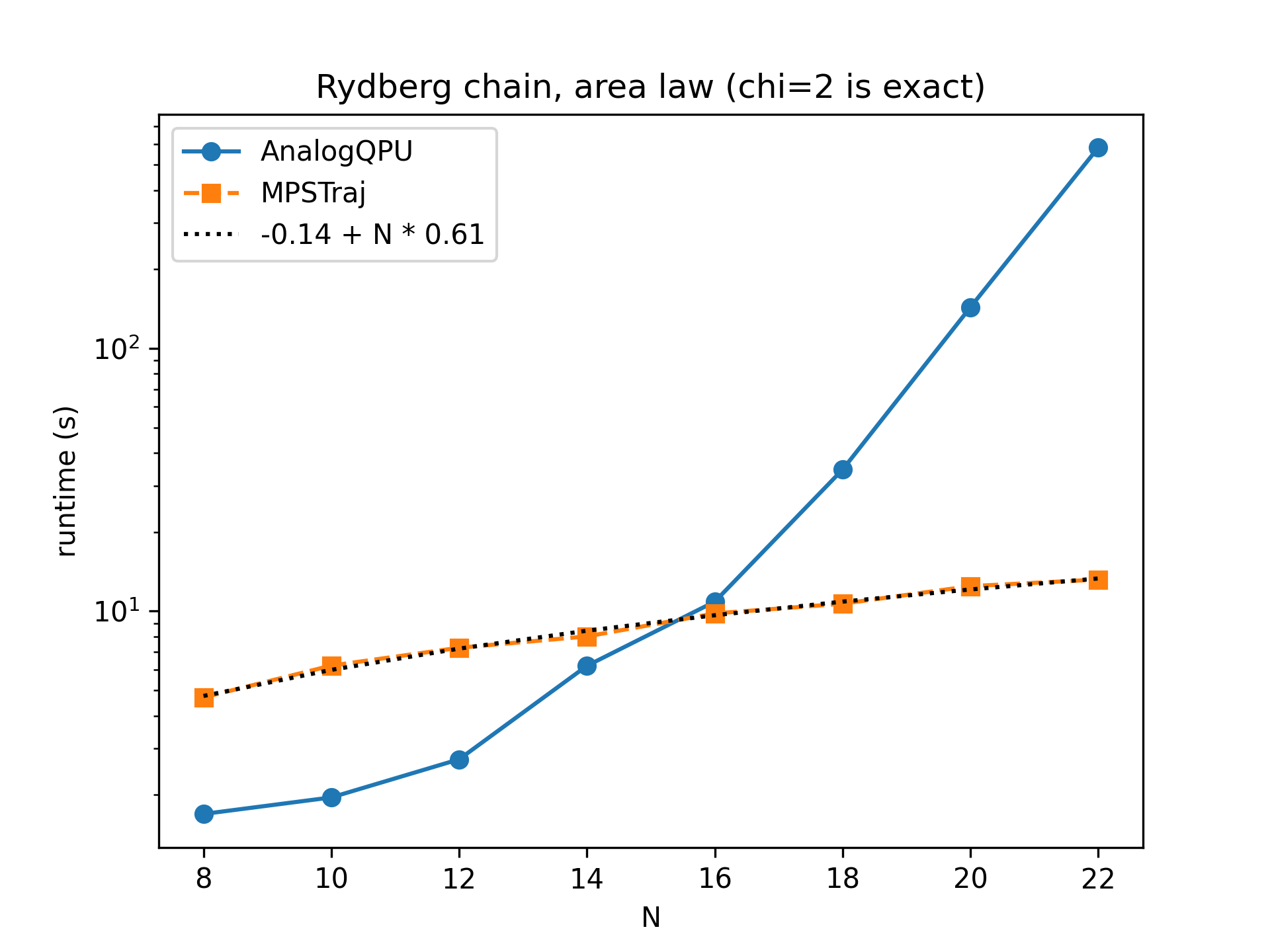
Comparison of runtimes for the emulation of a state preparation protocol in a 1D chain of \(N\) Rydberg atoms.

In the case of a 2D square lattice of atoms, the performances are still advantageous despite an increase of entanglement.

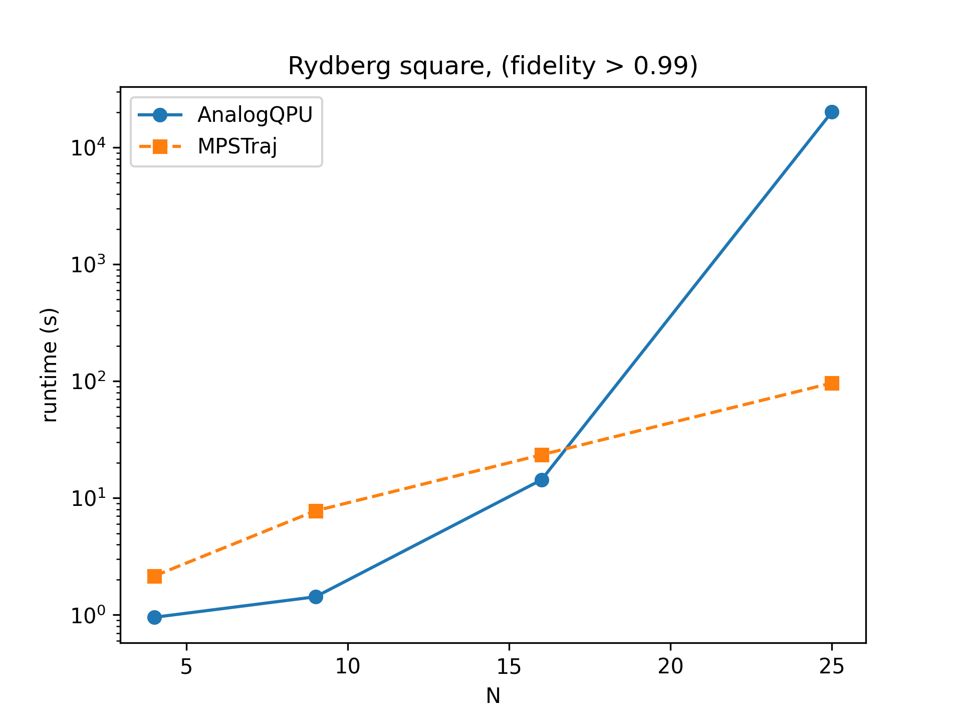
Comparison of runtimes for the emulation of a state preparation protocol in a 2D square lattice of \(N=L^2\) Rydberg atoms.

Bibliography

[Bonnes2014]

Bonnes L. and Läuchli A. M., Superoperators vs Trajectories for Matrix Product State Simulations of Open Quantum System: A Case Study, ArXiv:1411.4831.

[Breuer2007]

Breuer H.-P. and Petruccione F., The Theory of Open Quantum Systems, Oxford University Press, 2007.

[Daley2014]

Daley A. J., Quantum Trajectories and Open Many-Body Quantum Systems, Advances in Physics 63, 77 (2014), ArXiv:1405.6694.

[Percival1998]

Percival I., Quantum State Diffusion, Cambridge University Press, 1998.

[Plenio1998]

Plenio M. B. and Knight P. L., The Quantum-Jump Approach to Dissipative Dynamics in Quantum Optics, Rev. Mod. Phys. 70, 101 (1998), ArXiv:quant-ph/9702007.

[Schollwock2011]

Schollwöck U., The Density-Matrix Renormalization Group in the Age of Matrix Product States, Annals of Physics 326, 96 (2011), ArXiv:1008.477.

[Vovk2022]

Vovk T. and Pichler H., Entanglement-Optimal Trajectories of Many-Body Quantum Markov Processes, Phys. Rev. Lett. 128, 243601 (2022), ArXiv:2111.12048.