Creating noise models

Today’s quantum computers are imperfect, or “noisy”. One of the great challenges of quantum engineering is to understand the effect of this noise on the success, or failure, of a given quantum algorithm.

In this page we present the tools required to describe these imperfections in view of running simulations to predict their effects.

Overview and key concepts

Hardware Model

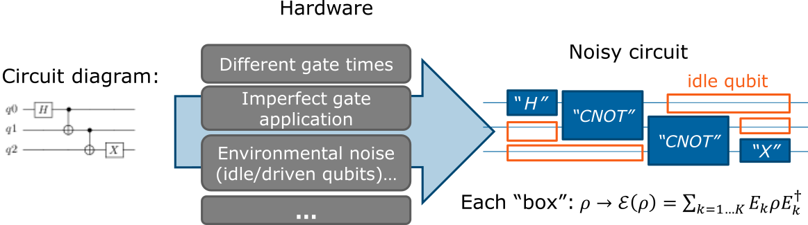
The sources of noise in quantum computing are imperfections of the quantum computer hardware. For example, idle qubits are not perfectly isolated from their environment, gates are applied within some error margin, etc. In Qaptiva, these noise sources are therefore described in a hardware model. A hardware model contains two kinds of information:

Specification of the gates: imperfections in gate applications, state preparation and measurement (‘gate’ is understood in the broad sense that includes state preparation and measurement), as well as how long each gate takes. This is stored in a gates specification.
The influence of the environment on qubits.

From a given circuit and hardware model, we produce a description of what happens when one runs this circuit on this hardware which is called a noisy circuit.

Noisy Circuit

A noisy circuit is a regular circuit that has been interpreted through the lens of a specific hardware model. It replaces the different elements of a circuit to add the defects caused by the hardware imperfections. The replaced elements are:

The initial pure state is replaced by a mixed state, represented by a density matrix, to take into account an imperfect state preparation.
Ideal gates are replaced by noisy gates. Mathematically, unitary operations are replaced by generalized quantum transformations called quantum channels.
Periods of inactivity for qubits (idling time) are replaced by an evolution under the influence of the environment, represented by another quantum channel.
Perfect projective measurements are replaced by noisy measurements, represented mathematically by Positive Operator-Valued Measurement (POVM).

The resulting circuit is made up of “boxes”, each of which describes an action on the density matrix of the qubits:

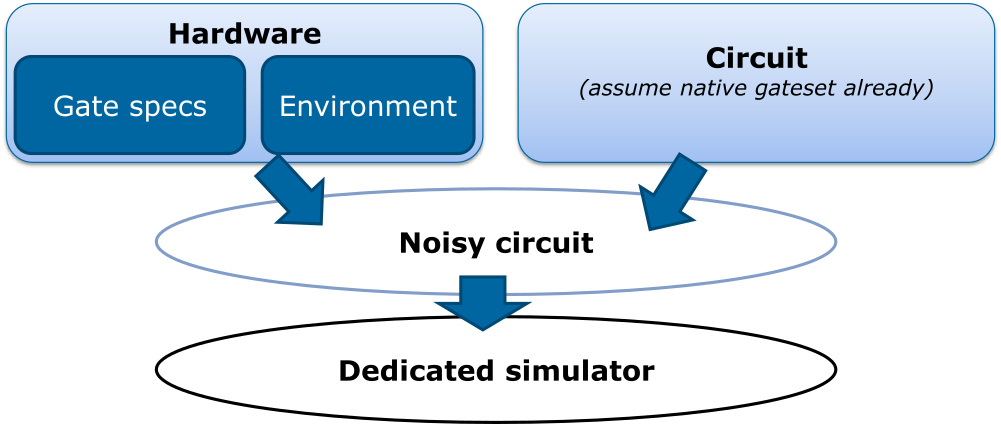
Finally, this noisy circuit is sent to one of the dedicated simulators of Qaptiva. Simulating a noisy circuit requires special-purpose simulators such as NoisyQProc.

The following diagram sums up Qaptiva’s workflow in dealing with noise simulation.

Defining a noise model in Qaptiva

Quantum Channels

The evolution of a quantum system under the influence of an environment is described by a quantum channel. A quantum channel \(\mathcal E\) is a transformation of the density matrices of the system \(\rho \rightarrow \mathcal E(\rho)\) which is:

linear
Completely Positive (CP)
Trace Preserving (TP) or trace reducing.

These properties are necessary to respect the axioms of quantum mechanics. They can be deduced from the fact that the system and the environment taken together must evolve under a Schrödinger equation. Linearity comes from the linearity of the Schrödinger equation. Complete positivity reflects the conservation of the positive semi-definite character of density matrices, even within any extension to a larger Hilbert space. The trace preserving or reducing property is a consequence of conservation of probabilities, i.e. of the unitarity of the Schrödinger equation. In the absence of measurements or leakage, quantum channels are trace preserving. The trace of a density matrix is then generally taken to be one.

Quantum channels are used to represent the action of noisy gates, or the action of the environment on qubits.

Quantum channels can come in different representations. The most common are implemented in the following classes:

QuantumChannelKraus the Kraus operators representation
QuantumChannelChoi the Choi-Jamiolkowski representation
QuantumChannelPTM the Pauli Transfer Matrix (PTM) representation
QuantumChannelChi the \(\chi\)-matrix representation

which all derive from QuantumChannel. While the Kraus representation ensures the CP character of the corresponding map, the PTM and the \(\chi\)-matrix representations do not necessarily have this property.

Quantum channels in any representation can be converted to any other representation. For instance, here we define a noisy Hadamard gate from its Kraus operators, and then cast it to a chi matrix representation:

import numpy as np
from qat.quops import QuantumChannelKraus

H_mat = np.array([[1, 1], [1, -1]])/np.sqrt(2)
p = 0.2
noisy_H = QuantumChannelKraus(kraus_operators=[np.sqrt(1-p)*H_mat, np.sqrt(p)*np.identity(2)],
                              name="noisy Hadamard")

noisy_H_chi = noisy_H.to_chi()
print(noisy_H_chi.matrix)

[[ 0.6+0.j  0.4+0.j  0.4+0.j -0.2+0.j]
 [ 0.4+0.j  0.4+0.j  0.4+0.j -0.4+0.j]
 [ 0.4+0.j  0.4+0.j  0.4+0.j -0.4+0.j]
 [-0.2+0.j -0.4+0.j -0.4+0.j  0.6+0.j]]

Roughly speaking, this noisy Hadamard corresponds to a Hadamard being applied only 80% of the time. The rest of the time, nothing (an identity matrix) is applied.

One can check important properties of quantum channels with the functions is_completely_positive(), is_unital(), is_trace_preserving() and is_trace_reducing(). These do not work with all representations, and convertion to a suitable representation may be needed first.

It is often interesting to use quantum channels which depend on a time duration. For example, the decoherence of a qubit depends on how long it is coupled to the environment. Such channels that depend on a parameter are called parametric quantum channel and are instances of ParametricQuantumChannel. For example, here we define the channel corresponding to pure dephasing with characteristic time \(T_{\phi} = 100 \mu\textrm{s}\) applied during \(5 \mu\textrm{s}\):

from qat.quops import QuantumChannel, ParametricPureDephasing

parametric_channel = ParametricPureDephasing(T_phi=100.)
channel = parametric_channel(5.0)

print(type(channel))

<class 'qat.quops.quantum_channels.QuantumChannelKraus'>

Examples of such channels are ParametricPureDephasing or ParametricAmplitudeDamping.

Note

Classes and functions about quantum channels are part of qat.quops. The following notebooks deal with quantum channels: Quantum channels, Parametric quantum channels, Noisy state preparation and measurement, Adding gate noise.

Defining Hardware models

Ideal gates

If we assume ideal gates, state preparation and measurement, only the coupling to the environment needs be taken into account. As a first approximation, one may want to apply some noise channel only when qubits are idle. To do that we need to inform the simulator of the time taken by each gate, which is part of the gates specification. For this simple case, we can make an instance of DefaultGatesSpecification with a dictionary of times as a parameter:

import numpy as np
from qat.hardware import DefaultGatesSpecification

gate_times = {"H": 1., "CNOT": 10., "RX": lambda ang: 10. + 0.3 * np.sin(ang)}
gates_spec = DefaultGatesSpecification(gate_times)

Parametric gates, like rotations, require a function of their parameter(s), as shown above.

We now need to choose a parametric noise channel for each qubit, and construct the hardware model:

from qat.hardware import HardwareModel
from qat.quops import ParametricPureDephasing

nbqubits = 3
T_dephas = [100., 85., 105.]

idle_noise = [ParametricPureDephasing(T_phi=T) for T in T_dephas]

hardware_model = HardwareModel(gates_spec, idle_noise=idle_noise)

We applied a pure dephasing noise channel with a different characteristic time on each qubit. This hardware model is ready to be given to a noisy circuit simulator.

In addition to idling time noise, one can add one or several noise channels after each gate application. For instance, here we add a dephasing noise after each application of the Hadamard gate:

from qat.quops import ParametricGateNoise

gate_noise = {"H": ParametricGateNoise(gate_spec, "H", [ParametricPureDephasing(T_phi=100.)])}

hardware_model = HardwareModel(gates_spec, gate_noise=gate_noise, idle_noise=idle_noise)

Using ParametricGateNoise is necessary for this to work. The channel is given as a parametric channel, because the exact noise channel applied will be deduced from the time duration of the gate.

Note

DefaultGatesSpecification already comes with a list of the most commonly used gates with zero execution time and no added noise. Therefore you do not need to list all gates you are going to use in the arguments. If it is produced without argument, it assumes gate execution time is zero, which effectively eliminate any idling time.

Noisy measurements and state preparation

Information about noisy measurements and state preparation is stored in the gates specifications. It is given as additional parameters to DefaultGatesSpecification:

state_prep = {k: np.array([[0.9, 0], [0, 0.1]]) for k in range(nbqubits)}
measure = {k: np.array([[0.1, 0], [0, 0.9]]) for k in range(nbqubits)}

gates_spec = DefaultGatesSpecification(gate_times, state_prep=state_prep, meas=measure)

The state preparation is described by a dictionary giving the density matrix in which each qubit should be prepared. Keys are indices of the qubits. As a result, the state of the register is prepared in a product state \(\rho_1 \otimes \rho_2 \otimes \ldots \otimes \rho_N\).

The measurement is described by a dictionary giving a POVM on each qubit. A POVM on a single qubit is a pair of positive semi-definite operators \(I - E\) and \(E\) with respective outcomes 0 and 1 (\(I\) is the identity). Our convention is therefore to provide only \(E\) (with outcome 1).

As a result, in the example above we asked that, for each qubit, state preparation should produce state \(|1\rangle\) 10% of the time, and measurement should fail to produce the correct answer 10% of the time.

Precise gates specification

For a perfect control on the noise description, Qaptiva allows to provide the precise operation produced by each gate. For this, we use the more general GatesSpecification class. We provide it with a dictionary mapping each gate to a quantum channel as follows:

H_mat = np.array([[1., 1.], [1., -1.]]) / np.sqrt(2.)
noisy_H = QuantumChannelKraus([np.sqrt(0.8) * H_mat, np.sqrt(0.2) * np.eye(2)], name="noisy Hadamard")
# noisy_CNOT = ...
# ...

quantum_channels = {"H": noisy_H, "CNOT": noisy_CNOT, "RX": lambda ang: noisy_RX(ang)}
gates_spec = GatesSpecification(gate_times, quantum_channels, state_prep=state_prep, meas=measure)

hardware_model = HardwareModel(gates_spec, idle_noise=idle_noise)

The provided channels completely overwrite the usual gates unitary operators. Noisy state preparation and measurement are described in the same way as above. The hardware model is produced as usualy.

Note

Unlike DefaultGatesSpecification, GatesSpecification requires information about every gate that is going to be used in circuits.

Predefined hardware models

A predefined hardware model can be obtained with make_depolarizing_hardware_model(). It only adds a depolarizing channel after each gate application.

Note

Classes and functions about hardware models are part of qat.hardware. The following notebooks deal with hardware models: Creating a custom hardware model, Using predefined hardware models. Noisy state preparation and measurements are covered in this notebook.

Running a noisy simulation

Running a noisy simulation is no different than running a simulation of an ideal quantum computer, except that the hardware model must be provided, and that a simulator which can handle noise must be used. Here is an example with the NoisyQProc simulator:

import numpy as np
from qat.lang import Program, H, CNOT, RX
from qat.qpus import NoisyQProc
from qat.hardware import HardwareModel, DefaultGatesSpecification
from qat.quops import ParametricAmplitudeDamping

nbqubits = 3
T_dephas = [100., 85., 105.]
gate_times = {"H": 1., "CNOT": 10., "RX": lambda ang: 10. + 0.3 * np.sin(ang)}
gates_spec = DefaultGatesSpecification(gate_times)
idle_noise = [ParametricAmplitudeDamping(T_1=T) for T in T_dephas]
hardware_model = HardwareModel(gates_spec, idle_noise=idle_noise)

qpu = NoisyQProc(hardware_model=hardware_model)

prog = Program()
reg = prog.qalloc(nbqubits)
H(reg[0])
CNOT(reg[0], reg[1])
CNOT(reg[1], reg[2])
RX(0.5 * np.pi)(reg[2])

job = prog.to_circ().to_job()
result = qpu.submit_job(job)

for sample in result:
   print("State %s, probability %s"%(sample.state, sample.probability))

State |0>, probability 0.2823812641674812
State |1>, probability 0.28238126416748116
State |10>, probability 0.08515564390712362
State |11>, probability 0.08515564390712364
State |100>, probability 0.036493408260790575
State |101>, probability 0.03649340826079059
State |110>, probability 0.09596968366460451
State |111>, probability 0.09596968366460455

More details on executing circuits can be found in Executing / Simulating quantum programs.