qat.qpus.SPD
- class qat.qpus.SPD(threshold: float = None, max_weight: int = None, max_size: int = None, max_x_weight: int = None, nprocs: int = 1, extract_clifford: bool = True, verbose: bool = False, disable_resource_management: bool = False, **kwargs)
Sparse Pauli Dynamics simulator QPU for noiseless quantum circuits.
Four truncation modes exist, and any combination of them can be applied:
Threshold: Set a threshold of acceptance for the coefficients of Pauli rows. Only Pauli rows above this threshold will be tracked.
Max weight: Set a maximum Hamming weight. Only Pauli rows with weight below this maximum will be kept.
Max size: Set a maximum number of Pauli rows. If exceeded, rows with the lowest coefficients will be discarded first.
Max X/Y support: Set a maximum number of X or Y terms allowed in each Pauli row.
Note
If none of the truncation methods (threshold, max_weight, max_size, or max_x_weight) are set, no truncation is performed and the simulation will be exact. This is generally much less efficient than using linear algebra-based methods.
- Parameters:
threshold (float, optional) – Threshold of acceptance for the coefficients of the Pauli rows.
max_weight (int, optional) – Maximum allowed Hamming weight of the Pauli rows.
max_size (int, optional) – Maximum allowed size of the PauliTableau throughout the simulation.
max_x_weight (int, optional) – Maximum allowed number of X and Y terms in the Pauli rows.
nprocs (int, optional) – Number of processors to use. Defaults to 1.
extract_clifford (bool, optional) – If True, performs Clifford recompilation. Defaults to True.
Mathematical description
This simulator computes expectation values of observables by studying their evolution of in the Pauli basis, going through the quantum circuit in reverse. This is equivalent to studying the time evolution of a system in the Heisenberg picture rather than in the Schrödinger picture.
This simulator aims to compute the expectation value of an observable, written as:
where \(\rho_0 = \ket{0 ... 0} \bra{0 ... 0}\), \(<\mathcal{O}>\) is an observable and \(U\) is a quantum circuit composed of Pauli rotations and Clifford gates:
Instead of applying the gates to the state vector like one normally would when using a simulator based on state vector representation, we place ourselves in the Heisenberg picture and apply the gates of the circuit to the observable in reverse order. The observable is stored in a Pauli tableau, \(<\mathcal{O}> = \sum_i c_i P_i\), which is simply a sparse representation of the observable in the Pauli basis.
The rules for appling a gate to the Paulis composing the observable are straightforward:
A Clifford gate maps a Pauli to another Pauli
Applying a Pauli rotation \(e^{-i \frac{\theta_j}{2} P_j}\) will yield
Essentially, the number of Paulis in the sparse representation of the observable increases exponentially with the number of rotations. We can then apply several truncation methods to efficiently approximate the observable and the expectation value. For more informations on the four truncation modes we provide, please refer to our user guide on SPD.
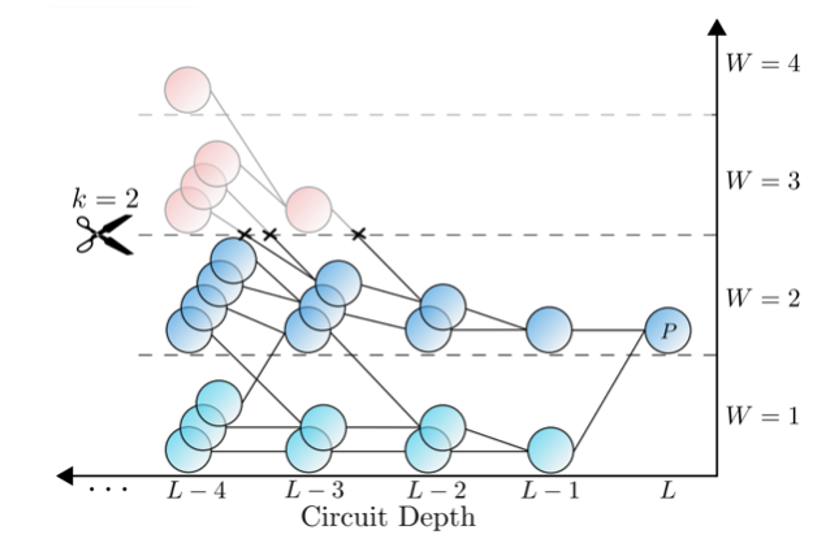
Graphical representation of the evolution of an observable through Pauli propagation. Here, the main observable branches out into different Paulis as we run through the circuit in reverse order. Here, a truncation method based on the Hamming weight of the Paulis is applied, by truncating all the Paulis whose weight is above the given maximum W=2.
Specs and use-cases
Specs:
Accepts Clifford gates and single-qubit rotations.
Very efficient simulation of near-Clifford quantum circuits (see use-cases below).
Accepts circuit with arbitrary connectivity.
Only computes expectation values of observables, samping cannot be performed.
Use cases:
Can simulate efficiently any near-Clifford circuit, i.e. circuits with a low number of non-Clifford gates, or where the rotations are close to multiples of \(\frac{\pi}{2}\). Instances include Trotter-like circuits [Begusic2023] or QAOA circuits [Begusic2025] with many Clifford gates.
Can simulate low-depth circuits with light-cones, or with locally scrambling distributions of gates [Angrisani2024].
Bibliography
Begušić, T., Fast classical simulation of evidence for the utility of quantum computing before fault tolerance. https://arxiv.org/abs/2306.16372.
Begušić, T., Fast and converged classical simulations of evidence for the utility of quantum computing before fault tolerance. Sci. Adv. 10, eadk4321 (2024), https://arxiv.org/abs/2308.05077.
Begušić, T., Simulating quantum circuit expectation values by Clifford perturbation theory. J. Chem. Phys. 162 (15): 154110 (2025), https://arxiv.org/abs/2306.04797.
Angrisani, A., Classically estimating observables of noiseless quantum circuits. https://arxiv.org/abs/2409.01706.
Begušić, T., Real-time operator evolution in two and three dimensions via sparse Pauli dynamics. PRX Quantum 6, 020302 (2025), https://arxiv.org/abs/2409.03097.