qat.qpus.Bdd

class qat.qpus.Bdd(threads=1, random_order=False)

Bdd simulator

Parameters

• threads (int, optional) – number of threads

• random_order (bool, optional) – if True, remap randomly the qubits

Mathematical description

Even though this simulator is named “BDD”, it is actually based on QMDDs (Quantum Multi-valued Decision Diagrams), which are a generalization of Binary Decision Diagrams to the quantum realm.

In classical computer science, BDDs are used to efficiently represent certain Boolean functions or circuits, and find application in circuit verification and compilation.

QMDDs can be used in a similar fashion in quantum computing. Like their classical counterparts, they can represent efficiently certain classes of quantum states and unitaries.

Our implementation of the BDD simulator is based on [Zulehner2017].

A QMDD is a recursive structure, dependent on an overall qubit ordering, consisting of nodes and weighted directed edges.

Each node is labeled by a qubit, and represents a sub-matrix/sub-vector of the overall unitary/vector which is represented. The size of this sub-matrix/sub-vector depends on the rank of the label qubit in the ordering. Each outgoing edge points to a lower-dimensional sub-matrix/sub-vector, represented by a node labeled with a qubit with higher rank in the order.

The sub-matrices/sub-vectors which are pointed to by outgoing edges are related to the values that the label qubit can take, and are defined, in the case of matrices, by the following convention:

Querying the value of an entry of a matrix from a QMDD representing it is carried out by following the decision path corresponding to the entry, visiting qubits according to their overall order, and multiplying edge weights along the way, up to a terminal node. See the “BDD example” figure below, for a concrete example.

The compression power of the representation comes from the fact that, in the case of identical sub-matrices, two edges can point to the same node, thereby avoiding redundant storage of information.

In the case of a vector, everything works the same, except that each node has only 2 outgoing edges.

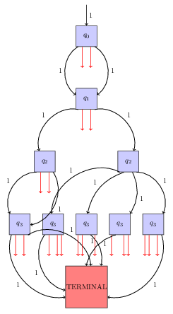
BDD example: QMDD representing a unitary matrix, generated by our simualator, from an actual quantum gate. Red arrow have weight 0. This particular diagram represents a unitary operator consisting of an identity on \(q_{0}\) and \(q_{1}\) tensored with a SWAP gate on the remaining qubits.

For example, one can check that the 16x16 matrix corresponding to the 4-qubit QMDD displayed on the <<BDD example>> figure is:

\[\begin{split}\left(\begin{array}{c|c} A & 0 \\ \hline 0 & A \end{array}\right)\end{split}\]

where \(A\) is:

\[\begin{split}A = \left(\begin{array}{c|c} \begin{array}{c|c} \begin{array}{c|c} 1 & 0 \\ \hline 0 & 1 \end{array} & (0) \\ \hline (0) & \begin{array}{c|c} 1 & 0 \\ \hline 0 & 1 \end{array} \end{array} & (0) \\ \hline (0) & \begin{array}{c|c} \begin{array}{c|c} 1 & 0 \\ \hline 0 & 0 \end{array} & \begin{array}{c|c} 0 & 0 \\ \hline 1 & 0 \end{array} \\ \hline \begin{array}{c|c} 0 & 1 \\ \hline 0 & 0 \end{array} & \begin{array}{c|c} 0 & 0 \\ \hline 0 & 1 \end{array} \end{array} \end{array} \right)\end{split}\]

In practice, the simulation works by forming and maintaining a QMDD for the state vector, and sequentially multiplying upon it the QMDDs corresponding to the unitaries of the circuit, according to the rules in [Zulehner2017].

Bibliography

Zulehner2017(1,2)

Alwin Zulehner and Robert Wille, https://arxiv.org/abs/1707.00865