qat.qpus.MPS
- class qat.qpus.MPS(bond_dimension: int = None, truncation_threshold: float = None, compression_method: str = 'SVD', fidelity: float = None, adaptative_strategy: str = 'naive', maximum_adaptative_bond_dimension: int = 1024, compute_fidelity: bool = False, progress_bar: bool = False, n_layers: int = 5, qubit_grouping: list = None, disable_resource_management: bool = False, nnize: bool = True, nnizer_kwargs: dict | None = None, seed: int | None = None, use_GPU: bool = False, svd_driver: str = 'gesdd', rsvd_iter: int = 2, **kwargs)
Matrix Product State simulator QPU for noiseless quantum circuits.
Three computation modes exist:
Fixed bond dimension mode: Setting a bond_dimension will compute the MPS and truncate any bond dimension above given bond_dimension value.
Truncation threshold mode: The bond dimension is set by discarding the singular values smaller than the truncation threshold.
Adaptative bond dimension mode: Setting a fidelity will ensure the final quantum state reaches a minima this fidelity value. The algorithm will adapt dynamically the bond dimension used throughout the calculation to ensure optimal bond dimension sizes and mnimal error. The fidelity set at the start is guaranteed. (Priority is given to this mode over the trunctation threshold mode if both are set).
Notes
MPS are well adapted to circuits with a 1D topology, but any circuit is supported. The NNizer plugin will be called automatically to transform any circuit into 1D topology.
If bond_dimension and fidelity are set to None, the algorithm will not truncate any bond dimension, and the simulation will be exact.
The initial state can be given as a string (e.g. “01+0”) or a numpy vector.
- Parameters:
bond_dimension (int, optional) – The bond dimension. Defaults to None, in which case no compression is done.
truncation_threshold (float, optional) – The truncation threshold when discarding singular values.
compression_method (str, optional) – The method of truncation to use. Several methods exist: - “SVD”: Truncation method based on SVD truncations. - “DMRG”: Truncation method based on the Density Matrix Renormalization Group (see Schollwoeck’s article). Default to “SVD”.
fidelity (float, optional) – If set, the truncation process will select automatically the maximum bond dimension allowed for each truncation such that the final fidelity of the state is higher or equal to input fidelity. This method is available only for the “SVD” compression method.
adaptative_strategy (str, optional) –
Strategy to adopt when selecting the fidelity of each quantum gate. The list of strategy includes:
”naive”: The fidelity goal is defined at the start of the simulation and is not dynamically updated.
”nearest”: The fidelity goal is updated from neighbour to neighbour. The first truncation fidelity computed updates the next nearest target truncation fidelity, while enforcing a total simulation fidelity higher than set input fidelity goal.
”global”: The fidelity is updated globally. Every computed truncation fidelity updates every remaining target truncation fidelity.
maximum_adaptative_bond_dimension (int, optional) – Maximum bond dimension the adaptative truncation scheme is allowed to reach. Falls back to maximum bond dimension truncation scheme if exceeded. In that case, the input fidelity is not guaranteed.
compute_fidelity (bool, optional) – If True, the fidelity will be stored for each truncation and each qubit, and added to the run metadata.
progress_bar (bool, optional) – If a progress bar should be displayed during the circuit simulation.
n_layers (int, optional) – The number of gates to be applied before a DMRG sweep. Defaults to 5. Available only for the “DMRG” compression method.
qubit_grouping (List[int], optional) – grouping of the qubits. E.g (4, 5, 2) for 3 groups with a total of 4+5+2=11 qubits. Defaults to None: no grouping, i.e (1, 1, …) (nqbits 1’s)
disable_resource_management (bool, optional) – If True, disable the resource management and set no limit on how much memory the QPU can use.
nnize (bool, optional) – whether to linearlize circuit before. Default to True.
nnizer_kwargs (dict, optional) – Dictionary of arguments to pass to the Nnizer plugin. Defaults to using the ‘atos’ method with window size 1. Refer to the Nnizer plugin documentation for more information.
seed (int, optional) – random number generator seed. Used in sampling mode with finite number of shots.
use_GPU (bool, optional) – If True, uses the torch implementation of the MPS to run the simulations on GPU. Defaults to False.
svd_driver (str, optional) – SVD algorithm used — “gesdd” (fast, default), “gesvd” (robust, stable), or “rsvd” (randomized approximation; much faster on GPU; only works with use_GPU).
rsvd_iter – (int, optional): Number of iterations for randomized SVD. Higher values give better accuracy but are slower. Defaults to 2. Only used if svd_driver is “rsvd”.
Mathematical description
This simulator represents the quantum state in the form of a matrix product state (MPS):
where \(\{M^{k,i_{k}}\}_{k=1\dots N}\) are matrices, with respective dimensions \(\left(\chi_{_{k-1}}, \chi_{_{k}}\right)\), consistent with matrix multiplication.
Essentially, applying operators (the quantum gates) increases bond dimensions throughout the simulation, and truncating these bond dimensions allows us to approximate the state. For more informations on the three truncation modes we provide, please refer to our user guide on MPS.
The \(\{\chi_{_{k}}\}_{k=1 \dots N}\) are called the bond dimensions. At the beginning of the simulation, with the state \(|0...0\rangle\), they are all equal to 1.
At all times, \(\chi_{_{0}} = \chi_{_{n}} = 1\).
The other bond dimensions can vary anywhere from 1 to exponentially large values, depending on the amount of entanglement within the system.
In fact, as a rule of thumb, if \(\mathcal{S}\) is the entanglement (von Neumann entropy of entanglement) of a state, then the maximum bond dimension will be of the order [Schollwoeck2010].
The simulation of slightly entangled quantum computations using MPS was first described by Guifré Vidal in [Vidal03]. Matrix Product States are a special case of tensor network states [Orus2014]. One could say that, within the MPS formulation, information has been relocalized into qubit-specific tensors, through factorization of the entire state vector. See [Vidal03] for more details.
The figure below gives the description of an MPS in the pictorial language of tensor networks, as a 1D-chain of rank-3 tensors: \(\{M^{k}\}_{k=1\dots N}\). For the sake of comparison, we also give the diagram corresponding to an entire amplitude vector, as used in the linalg simulator. (it is just a huge rank-N tensor)
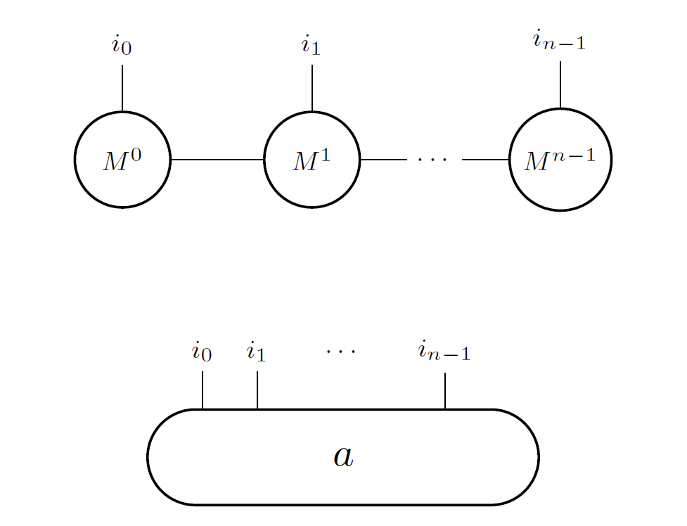
Graphical representation of the amplitude tensor, in the linear-algebra simulator (bottom) and in the MPS simulator (top).
In sample mode with a finite number of shots, samples are obtained efficiently using the OPES algorithm [Ballarin2024].
Specs and use-cases
Specs:
Accepts any one or two qubit unitary gate.
Very efficient simulation of slightly entangling quantum circuits (see use-cases below).
Accepts circuit with arbitrary connectivity (the compiler
qat.plugins.Nnizeris automatically used to respect the linear connectivity contraint of MPS).
Use cases:
Can simulate efficiently any circuit that does not produce much entanglement, when starting from \(|0 \dots 0\rangle\). Instances include QFT and arithmetic circuits, which are simulated much faster than with other simulators, and for more qubits, well beyond 50.
Can simulate Shor’s algorithm much faster than other simulators (but not with more qubits). This is because at some points during the execution of Shor’s algorithm, entanglement is actually rather low.
Bibliography
Orus, R., A Practical Introduction to Tensor Networks: Matrix Product States and Projected Entangled Pair States. Annals of Physics 349, 117–158 (2014), https://arxiv.org/abs/1306.2164.
Vidal, G., Efficient classical simulation of slightly entangled quantum computations. Phys. Rev. Lett. 91, 147902 (2003), https://arxiv.org/abs/quant-ph/0301063.
Schollwoeck, U., The density-matrix renormalization group in the age of matrix product states. Annals of Physics 326, 96–192 (2011), http://arxiv.org/abs/1008.3477.
Oliva, M., An entanglement-aware quantum computer simulation algorithm. Preprint at https://doi.org/10.48550/arXiv.2307.16870 (2023).
Ballarin, M. et al, Optimal sampling of tensor networks targeting wave function’s fast decaying tails. Preprint at https://arxiv.org/abs/2401.10330 (2024).