Simulation steps of QPEG

Global simulation sequence

This section explains the general algorithm behind QPEG. We then zoom in on each individual step.

State representation

In QPEG, the wave function \(|\psi \rangle\) is represented as a so-called grouped MPS. A standard Matrix Product State (MPS) is a list of matrices (formally tensors) with inner indices – indices between matrices of the MPS and outer indices – indices going outside of the MPS. The outer indices of an MPS are of dimension 2 (ie: they represent a single qubit). In a grouped MPS, we extend the standard MPS representation in two ways:

• Several qubits can be merged into qudits (specified with the qudit_grouping parameter).

• Qudits can then be grouped according to a grouping (specified with the groupings parameter), meaning that each matrix (or tensor) of the grouped MPS can have several outer indices (instead of one in a standard MPS).

Below is an example of an MPS being converted into a grouped MPS, according to a qudit_gouping of 2 (ie: 2 qubits per qudit) and a grouping of 2 (ie: 2 qudits per matrix of the grouped MPS). The number close to a given vertex indicates its dimensionality. The bond dimension of the grouped MPS is denoted as \(\chi\):

Here are a few more examples of groupings and qudit_grouping. The rightmost example represents a grouping that is equivalent to a single flat statevector of 9 qubits such as the one used in LinAlg.

Gate application

The goal of QPEG is to obtain a good approximation of the final wavefunction (that is, after the application of the circuit). To this aim, the gates of the circuit are grouped in so-called layers. A user may choose how the gates are put together in layers, with the parameter gates_per_layer. Once the gates are grouped in layers, the simulation proceeds by breaking the circuit down into groups of layers, called DMRG blocks. This can be done by using the parameter layers_per_dmrg. Reviewing the different parameters, here is an example:

For getting the above layering and DMRG blocking, one may use the following parameter values:

• gates_per_layer=2

• layers_per_dmrg=2

This means that as much as possible, gates will be assembled in layers of 2 and layers will be grouped in DMRG blocks of 2. Equivalent parameters would be:

• gates_per_layer=(2, 2, 2, 2, 1)

• layers_per_dmrg=(2, 2, 1)

After the application of each group of layers, an approximation of the intermediate wavefunction is computed (with various methods described below). After the last group is applied, one obtains the final wavefunction approximation and one can sample bitstrings from it or obtain the value of some observables.

Here is a diagram representing the basic steps of the simulator. The number of optimization steps, the number of layers (and the number of gates that are in each layer) can be defined by the user.

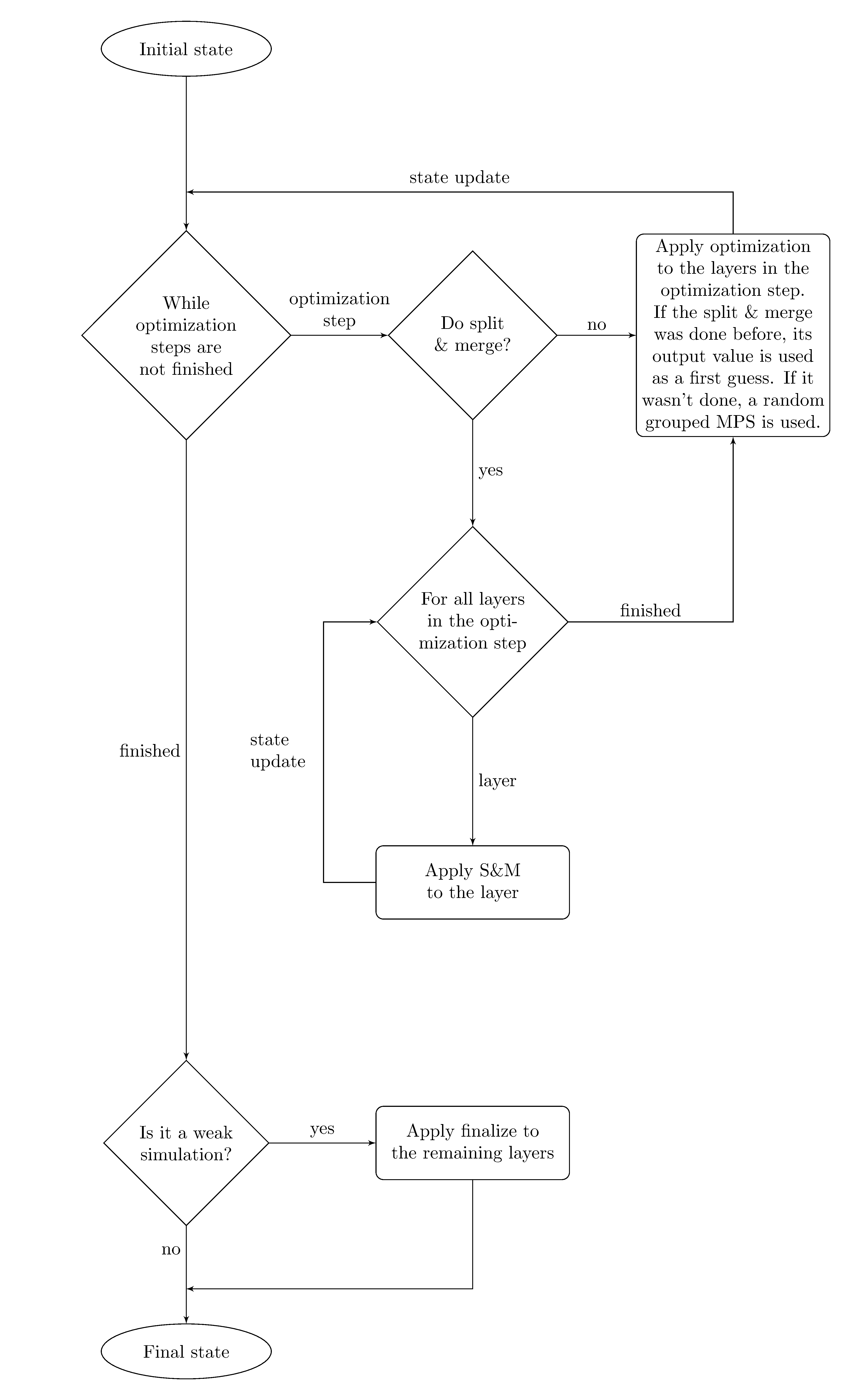
Note

While the option is available for the user to skip the DMRG phase and rely solely on the SVD phase, this is not a recommended course of action. For simplicity, this possibility isn’t represented in the above diagram.

Two methods for finding an approximate grouped MPS

There are two ways to find an approximate representation of the intermediate wavefunction: the DMRG and the SVD methods:

DMRG method

By default, this step is the only one used. The objective is to apply one or more layers to our quantum state, which is represented by a grouped MPS.

This is achieved by using a method called Density Matrix Renormalization Group (DMRG) [Schollwock2011]. Let us call target the first guess for the grouped MPS after the layers are applied to our system. The algorithm works with successive passes, each improving the value of one of the matrices of the target. One pass means contracting a tensor network such as:

The tensor resulting from the above contraction is a better candidate than the tensor that was removed from the target on the above diagram, and is now the new value of this MPS.

The above iteration is performed at least once per matrix. The number of times that such an optimization is done for each MPS is called the number of DMRG steps in QPEG, and can be configured with the dmrg_steps parameter.

SVD method

This step can be used either as a replacement or a preliminary stage to the DMRG step. Its objective is to apply a single layer to our quantum state, which is represented by a grouped MPS.

All the gates in the layer are applied sequentially and merged into the starting grouped MPS. This may compromise the shape of the tensors in the grouped MPS and therefore, the grouped MPS is put back in a proper grouping at the end of the layer. This is partly achieved by doing SVDs (Singular Value Decomposition), hence the name of this step.

The result of this step is mainly useful as a first guess for the target grouped MPS of an optimization step, however it can achieve decent results without DMRG afterward in specific cases.

Warning

this step was mainly intended for very structured circuits such as Google’s Sycamore experiment, and may perform poorly in other instances.

Strong vs weak simulation

Alternative:

Strong and weak refer to simulations whose computations give access to different types of information.

A strong simulation’s calculation provides information representing the full probability distribution of the output quantum states; and the result at the end of the simulation is drawn from this information. On the other hand, the calculation in a weak simulation only gives some samples of the output distribution, from which the result is constructed.

No weak simulation is yet implemented in QPEG, however a similar mode called single amplitude is available. Its output is the amplitude of a single bitstring, and a result obtained in this way has a better fidelity than a result obtained with a strong (default) simulation.

Note

This single amplitude mode, though it can be used for other use cases, has mainly been implemented as a proof of concept for being able to perform weak simulations of the Google Sycamore experiment.

Single amplitude mode & finalize simulation step

This mode can be used by setting the single_amplitude_mode parameter to True. By default, the amplitude measured is that of the bitstring 0. This can however be changed by adding a meta_data field to the submit Job object. An example can be found in the notebook on simulating the Sycamore experiment.

The overall simulation is changed when using this mode, and the circuit is split into three parts. Let us call these parts 1, 2, and 3.

Main part of the simulation:

A whole (strong) simulation is done on the left side with the part 1 of the circuit. Identically, a whole simulation is done on the right side with the part 3 of the circuit.

Final contraction step:

There only is a grouped MPS on the left, the part 2 of the circuit in the middle and a grouped MPS on the right. Such a tensor network looks like:

This tensor network is contracted, yielding the amplitude of the asked for bitstring.