QPEG use cases

QPEG has been heavily tested in two specific use cases:

• Simulating the Google sycamore experiment.

• Solving QAOA problems. Variational algorithms are thought to be good applications of NISQ computers, as they are less affected by fidelity decay. For the same reason, it seemed fitting to a non-exact simulator such as QPEG.

Sycamore experiment

The following section goes along with this notebook.

The main tools for reproducing the Google Sycamore experiment are under the module qat.qpeg.google. One can create a Circuit object that is a variation of the Sycamore experiment by using the following function:

qat.qpeg.google.create_google_sycamore_circuit(max_grid_height: int = 5, grid_width: int = 12, nb_layers: int = 20, fsim_theta: float = 1.5707963267948966, fsim_phi: float = 1.0, seed=2323, ordering='vertical', d_theta=0.0) → Circuit

Creates a Sycamore-like google circuit. Leaving default parameters reproduces the Google Sycamore circuit.

Parameters

• max_grid_height (int) – max number of qubits per column of the qubits grid (5=Google exp)

• grid_width (int) – number of columns of the qubits grid (12=Google exp)

• nb_layers (int) – number of layers of the circuit (20=Google exp)

• fsim_theta (float) – theta param for fSim gate

• fsim_phi (float) – phi param for fSim gate

• seed (int) –

Returns

Circuit

Note

This method is available as an application in Qaptiva Access.

Calling this function while leaving all parameters to default will generate a circuit of the same size as the ones used in the Google experiment.

Another function is more useful for running such a circuit with QPEG, that is generate_google_sycamore_parameters(). Similarly to the previous one, this function creates a Google-like circuit, but it also returns arguments which can then be used to instanciate a QPEG object.

qat.qpeg.google.generate_google_sycamore_parameters(single_amplitude_mode: bool = False, max_grid_height: int = 5, grid_width: int = 12, nb_layers: int = 20, fsim_theta: float = 1.5707963267948966, fsim_phi: float = 1.0, seed=2323) → tuple

Generates the circuit for the Google experiment, as well as the parameters needed to perform a simulation using QPEG. Leaving default parameters reproduces the Google Sycamore circuit.

Parameters

• single_amplitude_mode (bool) – whether or not to do the simulation in single amplitude mode

• max_grid_height (int) – max number of qubits per column of the qubits grid (5=Google exp)

• grid_width (int) – number of columns of the qubits grid (12=Google exp)

• nb_layers (int) – number of layers of the circuit (20=Google exp)

• fsim_theta (float) – theta param for fSim gate

• fsim_phi (float) – phi param for fSim gate

• seed (int) –

Returns

• a Circuit object

• a dict object containing the parameters for the QPEG simulation

Return type

Tuple

Note

This method is available as an application in Qaptiva Access.

The QPEG parameters returned by this function are intended to give good performance, (especially when at the default Google circuit or sizes close to it) and one should only need to change the bond_dimension parameter, though of course one can experiment with other parameters.

More in-depth examples are in the notebook, but a typical usage would look like:

from qat.qpus import QPEG
from qat.core import Observable
from qat.qpeg.google import generate_google_sycamore_parameters

circuit, parameters = generate_google_sycamore_parameters()
qpeg = QPEG(**parameters)

# the circuit may then be turned into a job and submitted
# this would be a strong simulation of the Google experiment, with a bond dimension of 1

The above example, with default parameters, is an example of strong simulation. A strong simulation’s calculation provides information representing the full probability distribution of the output quantum states; and the result at the end of the simulation is drawn from this information. On the other hand, the calculation in a weak simulation only gives some samples of the output distribution, from which the result is constructed.

QPEG does not yet support weak simulations, and strong simulations are its default mode. However, a variation of the weak simulation, that we call single amplitude mode, is available. More information on this mode is available here and here. An explanation of how this mode is used as a proof of concept for a weak simulation can be found in the notebook complementing this section.

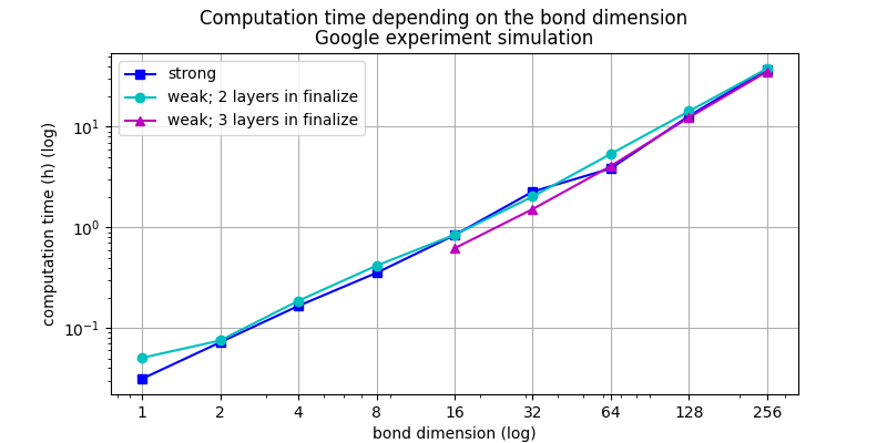
What is of most interest to us when simulating this type of experiment is not the result, but rather its fidelity and the time it took to get it. This type of information is available in the result’s meta data. Here would be a way to print the interesting fields:

# ...
# result = qpeg.submit(job)

print("Computation time:", result.meta_data["time"])
print("Fidelity of the circuit:", result.meta_data["fidelity"])
print("Mean fidelity per multi-qubit gate:", result.meta_data["fidelity_per_gate"])

An example is available in the notebook.

The graph below shows at what point our best simulation (magenta) reaches our estimation of the fidelity of the Google experiment (red, dashed).

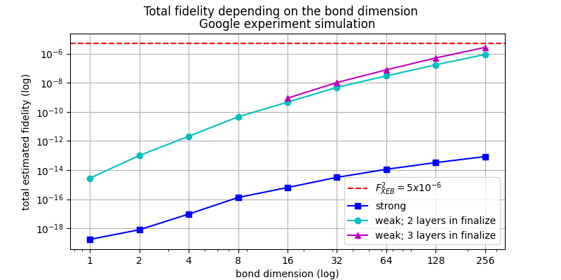
The cyan and magenta curves are called weak, as they are simulations using the single amplitude mode that are used as a proof of concept for a weak simulation. More information on this matter in the notebook. Our estimation of the fidelity of the experiment is \(F_{XEB}^2\), with \(F_{XEB}\) the value for the cross-entropy benchmarking in the Google paper. See [Zhou2020] for more information on fidelity estimation.

Generating the parameters with single_amplitude_mode=True, changing dmrg_sweeps to 2 and bond_dimension to a wanted value would result in generating a point on the above magenta curve.

QAOA

The following section goes along with this notebook.

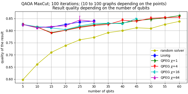
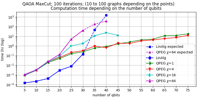
QPEG has been benchmarked on solving MaxCut problems with QAOA variational circuits. The following graphs show the quality of the result obtained with QPEG (compared to a perfect result of the problem) and the time taken by such simulations. These results are compared with LinAlg — Qaptiva’s exact simulator and with a random guess.

While one is encouraged to experiment with different parameters, QPEG performs well on QAOA problems with its default parameters. Most QPEG options (such as groupings, qudit_grouping, gates_per_layer, ….) were left to their default values when running the simulations that can be seen above. More information on how to use QPEG for solving QAOA problems can be found in this notebook.